Temperature adversely impacts strain measurements in many ways, though three are of primary concern:
• The device or object studied will almost always have a non-zero coefficient of thermal expansion. Unless compensated for, changes in temperature will cause the item to which the strain gauge is attached to expand or contract, which is then indicated as a change in strain.
• The materials of the strain gauge itself have a non-zero coefficient of thermal expansion. Changes in temperature will cause the strain gauge itself to expand or contract, independent of any strain in the part to which it is attached.
• The wiring and the strain gauge itself will have a non-zero Temperature Coefficient of Resistance. That is, as the temperature changes, the resistance of the strain gauge and connecting wires will change independently of any change in strain. (For example, copper wire resistance changes at approximately 3,900 ppm per °C (.393% /°C).)
Some texts treat the first two items as the same effect. After all, if the coefficients of expansion of the gauge and the item under test are the same, they will contract or expand at the same rates in response to a temperature change. In this case, a change in system temperature would not cause any change in the indicated strain, except that based on the gauge’s temperature coefficient of resistance.
It’s important to note that in some applications, it may be desirable or even critical that strain induced by temperature changes be noted. Imagine an application where a “hot section” turbine blade is being tested to ensure proper clearance between the blade tip and the surrounding shroud. It’s important to know how much the blade has elongated based upon temperature in addition to the centrifugal force of rotation. On the other hand, if the parameter of interest is really stress, or its close relative, force, any strain caused by temperature changes would induce a true error in the result. A strain gauge used to measure the “g” forces on a supersonic aircraft wing skin might see temperatures from -45°C to +200°C. If the g-force information was critical to not overstressing the wing, you’d certainly not want significant temperature-induced error. In a more simple case, the load cell used to measure the force placed on a postal scale should not induce errors simply because the scale is next to the window on a sunny summer day!
Most applications fall into the second category, where the key measurement parameter is really stress, and the ideal system would be not to recognize any changes caused by thermal expansion or contraction. Like most engineering challenges, there is more than one way to skin this proverbial cat. They are: (1) Calculate the error and eliminate it mathematically, (2) Match the strain gauge to the part, (3) Use an identical strain gauge in another leg of the bridge. We’ve previously covered how to eliminate it mathematically, so lets take a closer look at choices 2 and 3.
Match the Strain Gauge to the Part Tested
The use of different alloys/metals allows manufacturers to provide strain gauges designed to match the thermal expansion/contraction behavior of a wide variety of materials commonly subject to strain (and stress) testing. This type of gauge is referred to as a “Self Temperature Compensated” (or STC) strain gauge. These STC gauges are available from a variety of manufacturers and are specified for use on a wide assortment of part materials. As you might imagine, the more common a metal, the better the chances are there is an STC gage that matches. However, you may count on being able to find a good match for such materials as aluminum, brass, cast iron, copper, carbon steel, stainless steel, titanium and many more. Though the match between the STC gauge and the part under test may not be perfect, it will typically be accurate enough from freezing to well past the boiling point of water. For more details on the precise accuracy to expect, you should contact your strain gauge manufacturer.
Use an Identical Strain Gauge in Another Leg of the Bridge
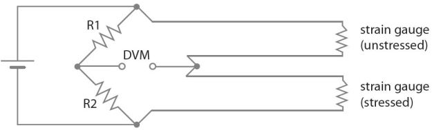
Due to the ratiometric nature of the Wheatstone bridge, a second, unstrained gauge (often referred to as a “dummy” gauge) placed in another leg of the bridge will compensate for temperature induced strain. Note that the dummy gauge should be identical to the “measuring” gauge and should be subject to the same environment.
Strain gauges tend to be small, and have short thermal time constants (i.e., their temperature changes very quickly in response to a temperature change around them), while the part under test may have substantial thermal mass and may change temperature slowly. For this reason, it is good practice to mount the dummy gauge adjacent to gauge being measured. However, it should be attached in such a way as not to be subjected to the induced strain of the tested part. In some cases, with relatively thin subjects and when measuring bending strain (as opposed to pure tensile or compressive strain), it may be possible to mount the dummy gauge on the opposite side of a bar or beam. In this case, the temperature impact of the gauges is eliminated and the scale factor of the output is effectively doubled.
Quarter, Half and Full Bridges
Strain gauges and measurement devices based upon strain gauges (e.g., load cells) can be configured in three different configurations. These are referred to as Quarter, Half and Full Bridges.
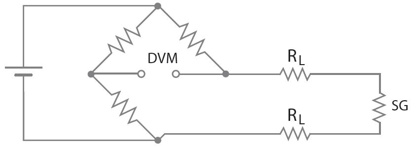
Quarter Bridge Strain Gauge
The quarter bridge gauge shown above is the simplest and probably most common strain gauge con-figuration (though some devices “based” on strain gauges are more likely to be provided in half or full bridge). The name “quarter” comes from the fact that in this configuration, the strain gauge represents one out of four, or one quarter of the resistors in the Wheatstone bridge. In this configuration, the user must supply the other three resistors.
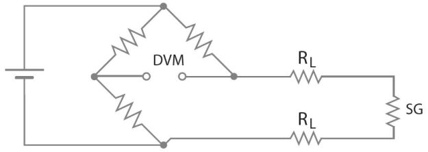
Half Bridge Strain Guage
In the half-bridge configuration, two resistors or half of the bridge are provided in the strain gauge itself. Half Bridge configurations have two advantages over the single bridge. First, they simply require the user to provide one less resistor. Second and more important, however, is the fact that most half bridge sensors automatically provide temperature compensation, made possible by having two identical gauges in the same side of the bridge.
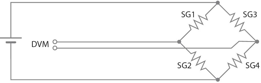
As you might expect, the full bridge sensor shown below provides all four resistors, in effect, providing the entire bridge. All the measurement system needs to provide is an excitation voltage and a differential analog input. Like the half-bridge configuration, most full bridge gauges are temperature compensated.
Learn more about measuring output from a strain gauge.

Full Bridge Strain Guage